]

Heterogeneous Materials

Homtools can be used to estimate the average mechanical response of a heterogeneous material by the way of Finite Element Analysis on a Representative Volume Element (RVE). It allows to compute the relationship between the average stress and the average strain, according to three different methods of localization: kinematic uniform boundary conditions (KUBC), periodic boundary conditions (PBC) and static uniform boundary conditions (SUBC). For all these methods, the average loading can be either the average stress or the average strain (or an independent combination of average strains and stresses components). The constitutive materials of the RVE can be either linear or non-linear and the analysis can be in small or finite-strain. The presence of interaction properties (such as contact and friction) is naturally taken into account.

Localisation boundary conditions

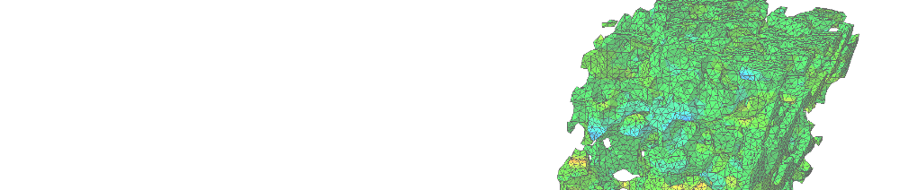
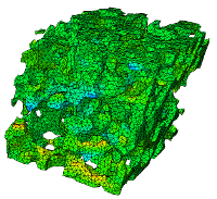
The following figures illustrate a simple 2D test case of a stiff elastic cylindrical filler in a soft elastic matrix, treated with the three available methods in Homtools: KUBC (Kinematic Uniform Boundary Conditions), PBC (Periodic Boundary Conditions), SUBC (Static Uniform Boundary Conditions).
PNG - 12.9 kb
PNG - 14.9 kb
PNG - 15.2 kb

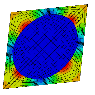
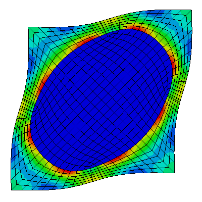
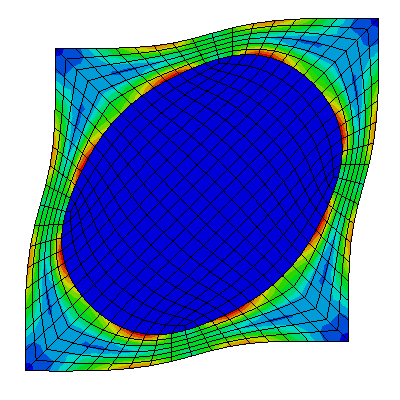
These methods require specific boundary conditions.

KUBC (click for a description)

This method consists in applying on the boundary the displacement field that would occur if the strain were uniform inside the RVE.

In small strains, the boundary conditions are :

\quad \vec{u} = < \bf{\varepsilon(\vec{u})}> \cdot \vec{OM}

in which :

-  \vec{u} is the displacement field,
-  \varepsilon(\vec{u}) is the strain field,
-  \vec{OM} is the position vector of the point  M on the boundary.
- <  \bullet > is the averaging operator over the RVE:  <  \bullet > = \frac{1}{\mbox{Vol}(V)} \displaystyle \int_V \; \bullet \; \mbox{d}V
-  \cdot is the inner product.

In finite strains, the boundary conditions are :

\quad \vec{u} = \left(< \bf{f}>-\bf{Id}\right)  \cdot \vec{OM}

in which :

- f is the deformation gradient,
-  \bf{Id} is the identity tensor.
-  \vec{OM} is the position vector of the point  M on the boundary in the reference configuration.
- <  \bullet > is the averaging operator over the RVE in the reference configuration:  <  \bullet > = \frac{1}{\mbox{Vol}(V)} \displaystyle \int_V \; \bullet \; \mbox{d}V
-  \cdot is the inner product.

There is no restriction concerning the use of this method, except that no rigid part must intersect the boundary (holes are permitted).
SUBC (click for a description)
This method consists in applying on the boundary the stress vector field that would occur if the stress were uniform inside the RVE.
In small strains, the boundary conditions are :

\quad \bf{\sigma} \bf{\cdot} \vec{n}} = <\bf{\sigma}>  \cdot \vec{n}

in which :

- \bf{\sigma} is the cauchy stress tensor,
-   \vec{n} is the outwarding normal.  <  \bullet > is the averaging operator over the RVE: <  \bullet > = \frac{1}{\mbox{Vol}(V)} \displaystyle \int_V \; \bullet \; \mbox{d}V
-  \cdot is the inner product.

In finite strains, the boundary conditions are :

\quad \bf{\pi} \bf{\cdot} \vec{n}} = <\bf{\pi}>  \cdot \vec{n}

in which :

- \bf{\pi} is the Piolla Kirchoff II stress tensor,
-   \vec{n} is the outwarding normal in the reference configuration. <  \bullet > is the averaging operator over the RVE in the reference configuration:  <  \bullet > = \frac{1}{\mbox{Vol}(V)} \displaystyle \int_V \; \bullet \; \mbox{d}V
-  \cdot is the inner product.

There is no restriction concerning the use of this method, except that no holes must intersect the boundary (rigid parts are permitted but a specific treatment is required).
PBC (click for a description)
The method is theoretically relevant for periodic media, which can be defined by a periodicity cell and the associated periodicity vector of translation. The periodic homogenisation process consists in assuming that the strains and stresses are periodic at the level of the periodicity cell (which is defined as the RVE). The periodicity of stresses and strains leads to specific periodic boundary conditions for the localisation problem on the RVE.
In small strains, the boundary conditions are :

\vect{u} - < \bf{\varepsilon(\vec{u})}>  \cdot \vec{OM} periodic and  \bf{\sigma} \cdot \vec{n}}  antiperiodic.

A quantity is said to be "periodic" (resp. "antiperiodic") when it takes the same value (resp. opposite value) at two opposite points on the boundary (one of them being the image of the other by translation of a periodicity vector).

In finite strains, the boundary conditions are :

\vect{u} - \left(< \bf{f}>-\bf{Id}\right)  \cdot \vec{OM} periodic and  \bf{\pi} \cdot \vec{n}}  antiperiodic. A quantity is in this case said to be "periodic" (resp. "antiperiodic") when it takes the same value (resp. opposite value) at two opposite points on the boundary (one of them being the image of the other by translation of a periodicity vector in the initial configuration).

There is no restriction concerning the use of this method (periodic holes and rigid parts intersecting the boundary are permitted but a specific treatment is required for the rigid parts).

The difficulty of applying these methods resides in the creation of the corresponding non classical boundary conditions, that can be written as linear constraints between the displacements at each point on the boundary of the RVE and the average strains.

In Homtools, we use Reference Points to prescribe the average loading and these constraints.

Reference Points to apply the average loading and the specific boundary conditions

The average strains are introduced as degrees of freedom of Reference Points and Homtools automatically generates the linear constraints (*equation) between these additionnal degrees of freedom and the displacements on the boundary of the RVE. Thanks to duality properties, the reaction forces at the Reference Points are the average stresses multiplied by the volume of the RVE. With this method, prescribing average strains or stresses becomes as easy as prescribing displacements or concentrated forces at a node. Furthermore, obtaining the relationship between the average strain and the average stress does not require any specific post-treatment.

For fiinte strain problems, the degrees of freedom of the Reference Points are the components of the average deformation gradient tensor and the reaction forces are the components of the avrage Piola-Kirchoff II stress tensor.

How to use Homtools

The main steps are :
- mesh the RVE
- in the "Interaction" module, create the Reference Points (2 for 2D problems in plane stress or strain or 3D problems in small strains, 3 for 3D problems in finite strains)
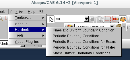
- in the "Interaction" module, choose "Homtools" in the drop off menu "Plug-in" and answer the questions.

- in the "Load" module, prescribe the average strains components or/and the stresses components by prescribing the degrees of freedom (dsplacements) or the nodal forces at the reference points.
- after solving the problem, in the "Vizualisation" module, you can obtain the effective response of the RVE by the postreatment of the displacements and yhe nodal forces at the Reference Points.

Check the following video to see the steps required to define a complete homogenization problem (in french).

Remarks


- for the method SUBC, no hole should intersect the boundary of the RVE (inconsistency of the method in this case). Furthermore, the displacement field is not unique for this method (rigid translations and rotations are not fixed)
- the method PBC is theoretically only relevant for periodic materials. The linear constraints couple the displacements at nodes on opposite faces of the boundary. The mesh of opposite faces must be identical: at each node of a face must correspond a node on the opposite face defined by translation of a periodicity vector. In Homtools, you must define the couple of faces together with a periodicity vectors : the mesh of the second set must result from the translation of the mesh of the first set according to the periodicity vector. You must repeat the operation as many times as necessary for all the couple of faces. Fot this method, the displacement field is not unique: the rigid translation is not fixed by the periodicity conditions and you can make the solution unique by fixing the dispalcements at a node in the RVE.